Time series forecasting with Auto ARMIA

Recently I came across some interesting algorithms and tools that can help with time series data analysis and forecasting. I found them very interesting from a developer’s perspective. So I think I need to write something about it.

How to do forecasting for sales, inventory and other time based data? I asked the question to some of my friends who are accountants. They said doing it manually with experience and based on the historical data. As developers, we like automating everything so computers can do the boring job with numbers. Here is what I found to how to do it in code from a developer’s perspective.

Time series forecasting with ARIMA

One of the most commonly used method for dealing with time series data is ARIMA, which stands for Autoregressive Integrated Moving Average. Here is what that means from wikipedia

In statistics and econometrics, and in particular in time series analysis, an autoregressive integrated moving average (ARIMA) model is a generalization of an autoregressive moving average (ARMA) model. Both of these models are fitted to time series data either to better understand the data or to predict future points in the series (forecasting). ARIMA models are applied in some cases where data show evidence of non-stationarity, where an initial differencing step (corresponding to the “integrated” part of the model) can be applied one or more times to eliminate the non-stationarity.

It is a complicated model and this is a nice article that explains what it is if you want to know more about it. Anyway, what we care about it how to use it and carry out the forecasting. So there are three params we need to pass to the function to work as p, d, q and for seasonal ARIMA, there are another set of these params as P, D, Q. We basically need to pass 6 params (p, d, q) and (P, D, Q) for seasonal ARIMA model to work. What are these parameters? They are explained in more detail here and here. How do I know what parameters we need to set? They are depending on the dataset and experts can tell by looking at the data and its statistical factors, it is well explained in this article. There is a lot of reading and math to learn to understand and know how to pick these parameters if you want to set it manually, like a pro:) Luckily there are tools and libraries available for people like me so they can be chosen automatically, so called ‘Grid Search’ method which is basically to try out all combinations and get the minimal AIC (Akaike Information Criteria). So this is what we are going to use for this post.

Importing Data

For demo purposes, I use Monthly milk production: pounds per cow. Jan 62 – Dec 75 as the input data. You can get the data from here. But the same process can be applied to most of time based data as well.

First we need to import libraries we need for this task. We need to install these packages by pip install if any of them are missing from the system.

import numpy as np
import pandas as pd
import statsmodels.api as sm
import matplotlib.pyplot as plt
from statsmodels.tsa.seasonal import seasonal_decompose
from pyramid.arima import auto_arima

Note that the magic module pyramid.arima which is the one we use to carry out this ‘grid search’ by trying out all combinations of different parameters and return the model that has the minimal AIC, automatically! Magic!

I downloaded the csv file. So use pandas to load the data into a data frame.

df = pd.read_csv('monthly-milk-production-pounds-p.csv')
df.columns = ['Month', 'Milk in pounds per cow']
#Remove the last row as it does not contain useful data
df.drop(168, axis=0, inplace=True)

#Convert the datetime string into real datetime type
df['Month'] = pd.to_datetime(df['Month'])

#Use the datetime column as the index
df.set_index('Month', inplace=True)
#Drop any empty value
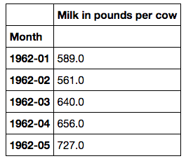
timeseries = df['Milk in pounds per cow'].dropna()

This is what the data looks like,

Visualise the data

Lets plot the data so we have some idea on the data we are working with.

timeseries.plot()
plt.show()

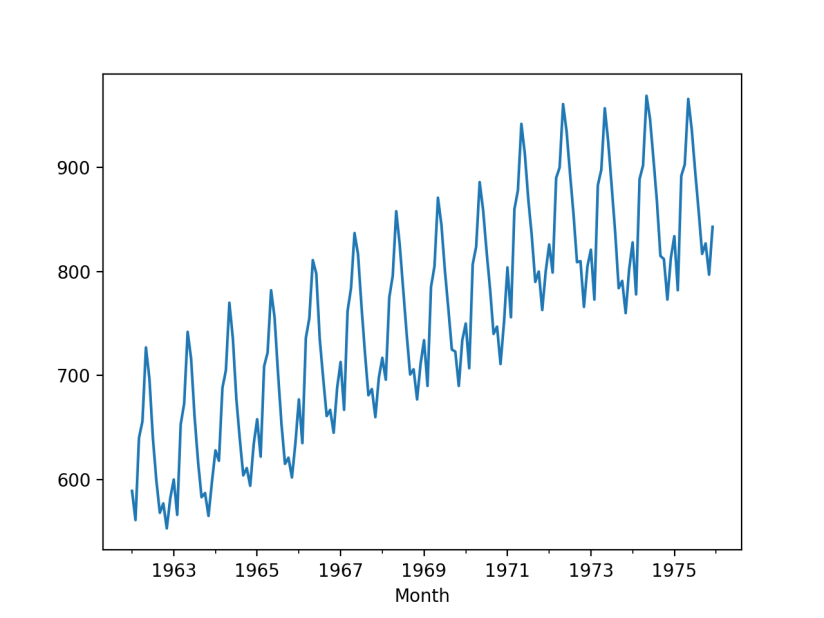
So we can see the trend and seasonality from the data, this indicates a seasonal ARIMA model to be used for forecasting.

decomp = seasonal_decompose(timeseries)
decomp.plot()
plt.show()

Here is the seasonal decomposition looks like.

We can see the trend and seasonality more clear in the breakdown components. Luckily we do not have to make it stationary before we can feed it into the auto_arima model.

Performing the Seasonal ARIMA with Pyramid-arima library

The pyramid-arima library is the magic tool we will use to perform the ‘grid search’ and automatically find the optimal p, d, q and P, D, Q parameters for training the model. Then we can train the model with our data.

model = auto_arima(
    timeseries,
    start_p=1,
    start_q=1,
    max_p=3,
    max_q=3,
    d=1,
    start_P=0,
    seasonal=True,
    m=12,
    D=1,
    trace=True,
    error_action='ignore',
    suppress_warnings=True,
    stepwise=True,
    transparams=False
    )
print('AIC is ' + str(model.aic()))

Here is the API doc for auto_armia function for each parameter. Here is the output,

You can see it found the optimal parameters p=0, d=1, q=3 and P=0, D=1, Q=2 and 12 for the seasonal order. It is loaded with this set of parameters at the end of the search so it ready for training.

Train the model

Just like training other models, we need to split our dataset into a training set and a test set so we can verify the performance. In this case, we will have training data from 1962-01 to 1973-07 and use the remaining rows for test set.

# #split the data set into training set and test set
train = timeseries.loc['1962-01':'1973-07']
test = timeseries.loc['1973-08':]

Training the model is just a single line of code.

model.fit(train)

Preform forecasting

We will let the model make prediction for next 29 months which match our test set data so we can compare with the actual test data.

future_forecast = model.predict(n_periods=29)
print(future_forecast)

Here is the forecast data,

We can compare the forecast data against the actual test data in the same plot.

future_forecast = pd.DataFrame(future_forecast, index=test.index, columns=['Prediction'])
pd.concat([test, future_forecast], axis=1).plot()

plt.show()

That is what it looks like side by side with the test data which is the actual historical data.

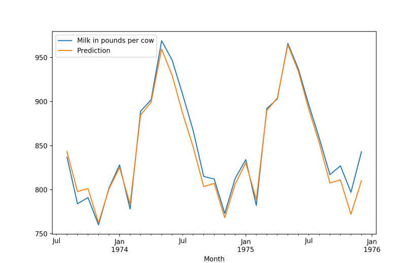
We can see it looks pretty good.

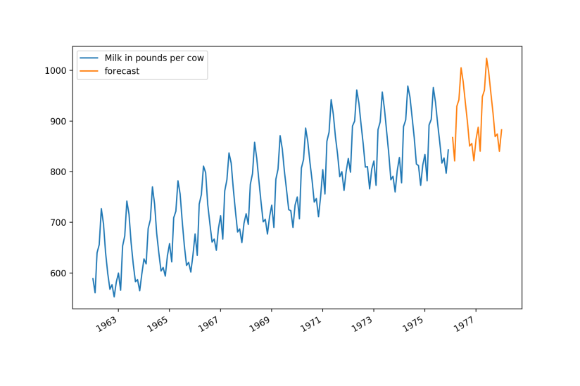
Predict more! We will train the model with the full dataset and use it to predict the next 24 months data.

#fit the model with the full historical data
model.fit(df)
#predict the next 24 month data
future_dates = [df.index[-1] + DateOffset(months=x) for x in range(1,26) ]
future_dates_df = pd.DataFrame(index=future_dates[1:],columns=df.columns)

future_dates_df['forecast'] = model.predict(n_periods=(24))
future_df = pd.concat([df,future_dates_df])
future_df[['Milk in pounds per cow', 'forecast']].plot(figsize=(12, 8))
plt.show()

Here is the data looks like visually.

Thoughts

Overall it looks pretty good considering how much effort we put in. Only a few lines of code, we can have a automated forecasting done quickly and it looks pretty good. However, ARIMA does not apply to all time series data and to get the seasonal ARIMA to work well, it requires quite long period of data which might not be available to newly founded organisations. I tried with daily data and it does not seem to work well. So I guess there are some limitations on this model. Anyway, it is relatively easy to use with auto ARIMA library and you can get good quality result fairly quickly. That said, manual analysis and adjustment is still needed but it can be a good starting point for further analysis. You can find the full source code in Github here.